Hierarchical forecasting

In forecasting, we often find ourselves in need of forecasts for both lower- and higher (temporal) granularities, such as product demand forecasts but also product category or product department forecasts. These granularities can be formalized through the use of a hierarchy. In hierarchical forecasting, we create forecasts that are coherent with respect to a pre-specified hierarchy of the underlying time series.

With TimeGPT, we can create forecasts for multiple time series. We can subsequently post-process these forecasts using hierarchical forecasting techniques of HierarchicalForecast.

1. Import packages

First, we import the required packages and initialize the Nixtla client.

import pandas as pd
import numpy as np

from nixtla import NixtlaClient

nixtla_client = NixtlaClient(
    # defaults to os.environ.get("NIXTLA_API_KEY")
    api_key = 'my_api_key_provided_by_nixtla'
)

👍

Use an Azure AI endpoint

To use an Azure AI endpoint, set the base_url argument:

nixtla_client = NixtlaClient(base_url="you azure ai endpoint", api_key="your api_key")

2. Load data

We use the Australian Tourism dataset, from Forecasting, Principles and Practices which contains data on Australian Tourism. We are interested in forecasts for Australia’s 7 States, 27 Zones and 76 Regions. This constitutes a hierarchy, where forecasts for the lower levels (e.g. the regions Sidney, Blue Mountains and Hunter) should be coherent with the forecasts of the higher levels (e.g. New South Wales).

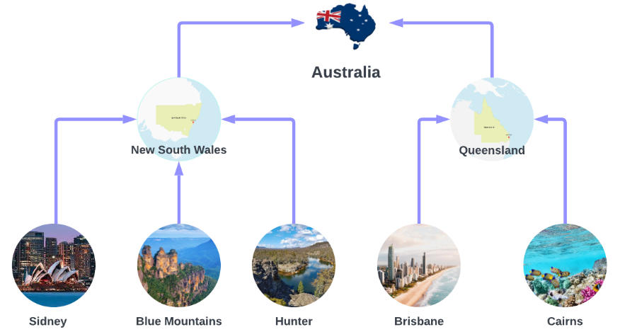
The dataset only contains the time series at the lowest level, so we need to create the time series for all hierarchies.

Y_df = pd.read_csv('https://raw.githubusercontent.com/Nixtla/transfer-learning-time-series/main/datasets/tourism.csv')
Y_df = Y_df.rename({'Trips': 'y', 'Quarter': 'ds'}, axis=1)
Y_df.insert(0, 'Country', 'Australia')
Y_df = Y_df[['Country', 'Region', 'State', 'Purpose', 'ds', 'y']]
Y_df['ds'] = Y_df['ds'].str.replace(r'(\d+) (Q\d)', r'\1-\2', regex=True)
Y_df['ds'] = pd.to_datetime(Y_df['ds'])

Y_df.head(10)

C:\Users\ospra\AppData\Local\Temp\ipykernel_28980\3753786659.py:6: UserWarning: Could not infer format, so each element will be parsed individually, falling back to `dateutil`. To ensure parsing is consistent and as-expected, please specify a format.
  Y_df['ds'] = pd.to_datetime(Y_df['ds'])

The dataset can be grouped in the following hierarchical structure.

spec = [
    ['Country'],
    ['Country', 'State'], 
    ['Country', 'Purpose'], 
    ['Country', 'State', 'Region'], 
    ['Country', 'State', 'Purpose'], 
    ['Country', 'State', 'Region', 'Purpose']
]

Using the aggregate function from HierarchicalForecast we can get the full set of time series.

Note

You can install hierarchicalforecast with pip:

Shell

pip install hierarchicalforecast

from hierarchicalforecast.utils import aggregate

Y_df, S_df, tags = aggregate(Y_df, spec)
Y_df = Y_df.reset_index()

Y_df.head(10)

We use the final two years (8 quarters) as test set.

Y_test_df = Y_df.groupby('unique_id').tail(8)
Y_train_df = Y_df.drop(Y_test_df.index)

3. Hierarchical forecasting with TimeGPT

First, we create base forecasts for all the time series with TimeGPT. Note that we set add_history=True, as we will need the in-sample fitted values of TimeGPT.

We will predict 2 years (8 quarters), starting from 01-01-2016.

timegpt_fcst = nixtla_client.forecast(df=Y_train_df, h=8, freq='QS', add_history=True)

INFO:nixtla.nixtla_client:Validating inputs...
INFO:nixtla.nixtla_client:Preprocessing dataframes...
INFO:nixtla.nixtla_client:Calling Forecast Endpoint...
INFO:nixtla.nixtla_client:Calling Historical Forecast Endpoint...

📘

Available models in Azure AI

If you are using an Azure AI endpoint, please be sure to set model="azureai":

nixtla_client.forecast(..., model="azureai")

For the public API, we support two models: timegpt-1 and timegpt-1-long-horizon.

By default, timegpt-1 is used. Please see this tutorial on how and when to use timegpt-1-long-horizon.

timegpt_fcst_insample = timegpt_fcst.query("ds < '2016-01-01'")
timegpt_fcst_outsample = timegpt_fcst.query("ds >= '2016-01-01'")

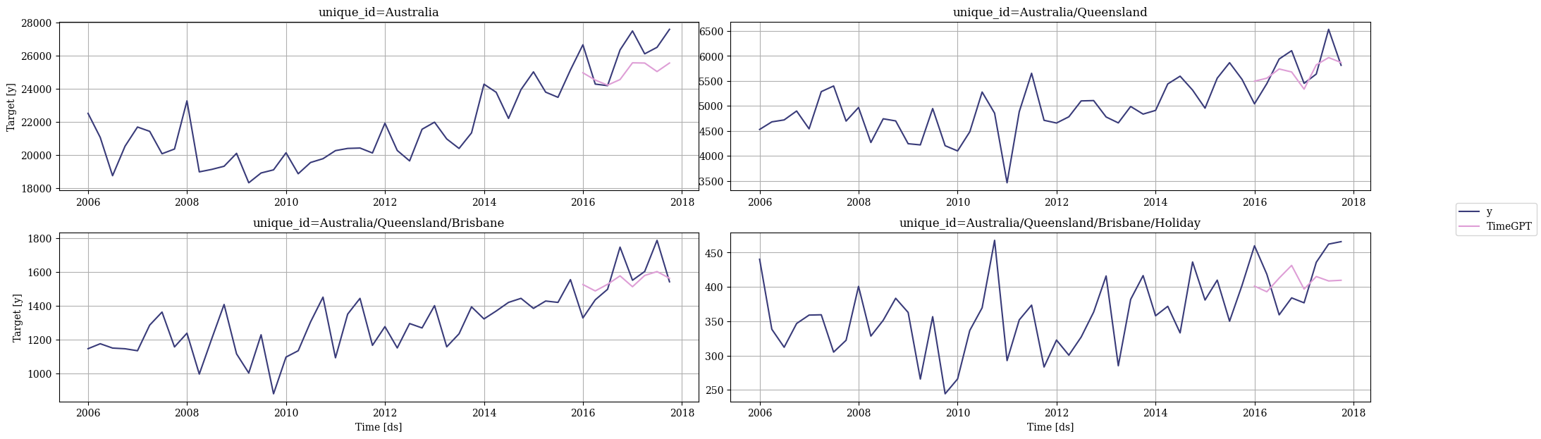
Let’s plot some of the forecasts, starting from the highest aggregation level (Australia), to the lowest level (Australia/Queensland/Brisbane/Holiday). We can see that there is room for improvement in the forecasts.

nixtla_client.plot(
    Y_df, 
    timegpt_fcst_outsample, 
    max_insample_length=4 * 12, 
    unique_ids=['Australia', 'Australia/Queensland','Australia/Queensland/Brisbane', 'Australia/Queensland/Brisbane/Holiday']
)

We can make these forecasts coherent to the specified hierarchy by using a HierarchicalReconciliation method from NeuralForecast. We will be using the MinTrace method.

from hierarchicalforecast.methods import MinTrace
from hierarchicalforecast.core import HierarchicalReconciliation

reconcilers = [
    MinTrace(method='ols'),
    MinTrace(method='mint_shrink'),
]
hrec = HierarchicalReconciliation(reconcilers=reconcilers)

Y_df_with_insample_fcsts = Y_df.copy()
Y_df_with_insample_fcsts['ds'] = Y_df_with_insample_fcsts['ds'].astype(str)
Y_df_with_insample_fcsts = timegpt_fcst_insample.merge(Y_df_with_insample_fcsts)
Y_df_with_insample_fcsts = Y_df_with_insample_fcsts.set_index('unique_id')

Y_rec_df = hrec.reconcile(Y_hat_df=timegpt_fcst_outsample.set_index('unique_id'), Y_df=Y_df_with_insample_fcsts, S=S_df, tags=tags)

Again, we plot some of the forecasts. We can see a few, mostly minor differences in the forecasts.

nixtla_client.plot(
    Y_df, 
    Y_rec_df.reset_index(), 
    max_insample_length=4 * 12, 
    unique_ids=['Australia', 'Australia/Queensland','Australia/Queensland/Brisbane', 'Australia/Queensland/Brisbane/Holiday']
)

Let’s numerically verify the forecasts to the situation where we don’t apply a post-processing step. We can use HierarchicalEvaluation for this.

from hierarchicalforecast.evaluation import HierarchicalEvaluation

def rmse(y, y_hat):
    return np.mean(np.sqrt(np.mean((y-y_hat)**2, axis=1)))

eval_tags = {}
eval_tags['Total'] = tags['Country']
eval_tags['Purpose'] = tags['Country/Purpose']
eval_tags['State'] = tags['Country/State']
eval_tags['Regions'] = tags['Country/State/Region']
eval_tags['Bottom'] = tags['Country/State/Region/Purpose']
eval_tags['All'] = np.concatenate(list(tags.values()))

evaluator = HierarchicalEvaluation(evaluators=[rmse])
evaluation = evaluator.evaluate(
        Y_hat_df=Y_rec_df.rename(columns={'y': 'TimeGPT'}), Y_test_df=Y_test_df.set_index('unique_id'),
        tags=eval_tags, Y_df=Y_train_df.set_index('unique_id')
)
evaluation = evaluation.drop(labels='Overall', level='level')
evaluation.columns = ['Base', 'MinTrace(ols)', 'MinTrace(mint_shrink)']
evaluation = evaluation.map('{:.2f}'.format)

evaluation

We made a small improvement in overall RMSE by reconciling the forecasts with MinTrace(ols), and made them slightly worse using MinTrace(mint_shrink), indicating that the base forecasts were relatively strong already.

However, we now have coherent forecasts too - so not only did we make a (small) accuracy improvement, we also got coherency to the hierarchy as a result of our reconciliation step.

References

• Hyndman, Rob J., and George Athanasopoulos (2021). “Forecasting: Principles and Practice (3rd Ed)”