Forecasting Energy Demand
This tutorial is based on an energy consumption forecasting scenario where we make a 4-day forecast of in-zone energy consumption.
Here, we use a subset of the PJM Hourly Energy Consumption dataset, focusing on in-zone consumption, where electricity is both generated and consumed within the same transmission zone. The dataset consists of hourly data from October 1, 2023, to September 30, 2024, covering five representative areas to capture hourly energy demand patterns.
In this experiment, we show that using TimeGPT delivers significant improvements over using a state-of-the-art deep learning model like N-HiTS in a just a few lines of code:
- MAE of TimeGPT is 18.6% better than N-HiTS
- sMAPE of TimeGPT is 31.1% better than N-HiTS
- TimeGPT generated predictions in 4.3 seconds, which is 90% faster than training and predicting with N-HiTS.
The following tutorial explore all the steps in detail to reproduce these results so that you can apply TimeGPT in your own project.
Initial setup
First, we load the required packages for this experiment.
import time
import requests
import pandas as pd

from nixtla import NixtlaClient

from utilsforecast.losses import mae, smape
from utilsforecast.evaluation import evaluate
Of course, we need an instance of NixtlaClient to use TimeGPT.
nixtla_client = NixtlaClient(
    # defaults to os.environ.get("NIXTLA_API_KEY")
    api_key = 'my_api_key_provided_by_nixtla'
)
Use an Azure AI endpoint
To use an Azure AI endpoint, remember to set also the
base_urlargument:
nixtla_client = NixtlaClient(base_url="you azure ai endpoint", api_key="your api_key")
Read the data
Here, we load in the inbound energy transmission time series.
df = pd.read_csv('https://raw.githubusercontent.com/Nixtla/transfer-learning-time-series/refs/heads/main/datasets/pjm_in_zone.csv')
df['ds'] = pd.to_datetime(df['ds'])
df.groupby('unique_id').head(2)
| unique_id | ds | y | |
|---|---|---|---|
| 0 | AP-AP | 2023-10-01 04:00:00+00:00 | 4042.513 |
| 1 | AP-AP | 2023-10-01 05:00:00+00:00 | 3850.067 |
| 8784 | DOM-DOM | 2023-10-01 04:00:00+00:00 | 10732.435 |
| 8785 | DOM-DOM | 2023-10-01 05:00:00+00:00 | 10314.211 |
| 17568 | JC-JC | 2023-10-01 04:00:00+00:00 | 1825.101 |
| 17569 | JC-JC | 2023-10-01 05:00:00+00:00 | 1729.590 |
| 26352 | PN-PN | 2023-10-01 04:00:00+00:00 | 1454.666 |
| 26353 | PN-PN | 2023-10-01 05:00:00+00:00 | 1416.688 |
| 35136 | RTO-RTO | 2023-10-01 04:00:00+00:00 | 69139.393 |
| 35137 | RTO-RTO | 2023-10-01 05:00:00+00:00 | 66207.416 |
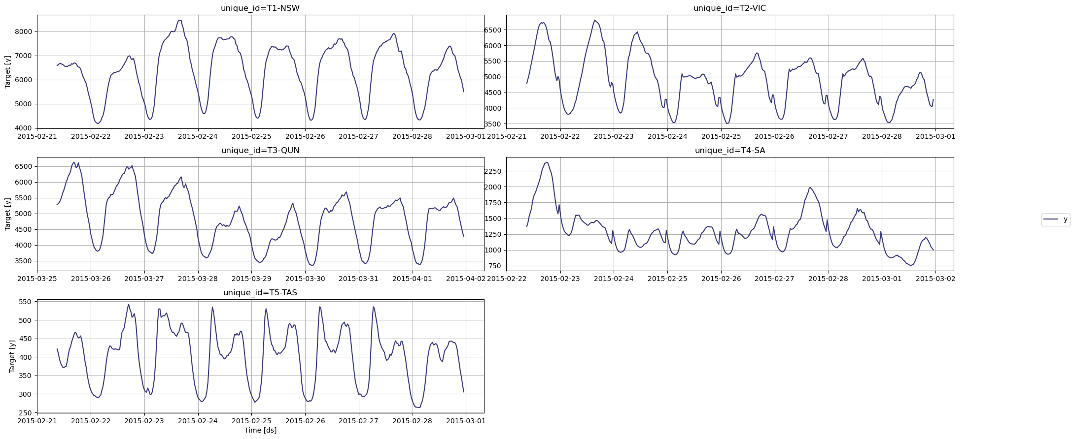
Let’s plot our series to see what it looks like.
nixtla_client.plot(
    df,
    max_insample_length=365,
)

We can see clear sesaonal pattern in all of our series. It will be interesting to see how TimeGPT handles this type of data.
Forecasting with TimeGPT
Splitting the data
The first step is to split our data. Here, we define an input DataFrame to feed to the model. We also reserve the last 96 time steps for the test set, so that we can evaluate the performance of TimeGPT against actual values.
For this situation, we use a forecast horizon of 96, which represents four days, and we use an input sequence of 362 days, which is 8688 time steps.
test_df = df.groupby('unique_id').tail(96)                                                             # 96 = 4 days (96 *  1 day/24h )

input_df = df.groupby('unique_id').apply(lambda group: group.iloc[-1104:-96]).reset_index(drop=True)   # 1008 = 42 days (1008 * 1 day/24h)
Forecasting
Then, we simply call the forecast method. Here, we use fine-tuning and specify the mean absolute error (MAE) as the fine-tuning loss. Also, we use the timegpt-1-long-horizon since we are forecasting the next two days, and the seasoanl period is one day.
start = time.time()

fcst_df = nixtla_client.forecast(
    df=input_df,
    h=96,
    level=[90],                        # Generate a 90% confidence interval
    finetune_steps=10,                 # Specify the number of steps for fine-tuning
    finetune_loss='mae',               # Use the MAE as the loss function for fine-tuning
    model='timegpt-1-long-horizon',    # Use the model for long-horizon forecasting
    time_col='ds',
    target_col='y',
    id_col='unique_id'
)

end = time.time()

timegpt_duration = end - start

print(f"Time (TimeGPT): {timegpt_duration}")
Available models in Azure AI
If you are using an Azure AI endpoint, please be sure to set
model="azureai":
nixtla_client.forecast(..., model="azureai")For the public API, we support two models:
timegpt-1andtimegpt-1-long-horizon.By default,
timegpt-1is used. Please see this tutorial on how and when to usetimegpt-1-long-horizon.
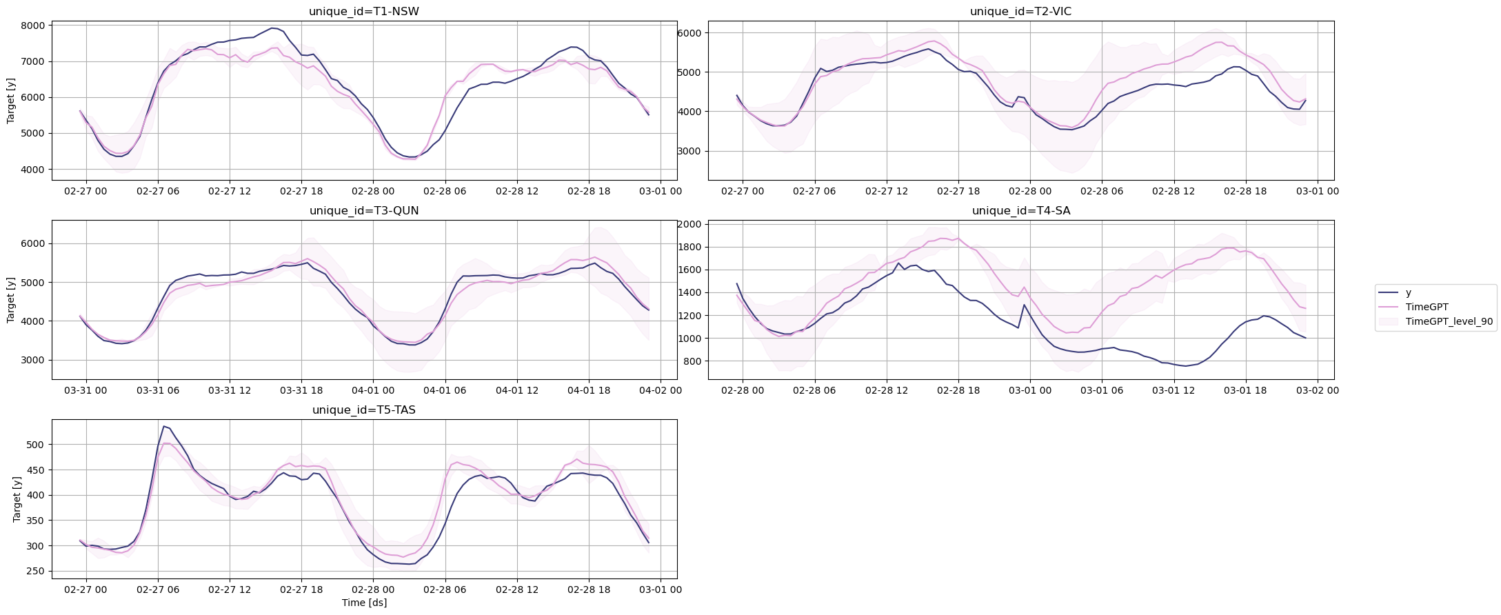
TimeGPT was done in 4.3 seconds! We can now plot the predictions against the actual values of the test set.
nixtla_client.plot(test_df, fcst_df, models=['TimeGPT'], level=[90], time_col='ds', target_col='y')

Evaluation
Now that we have predictions, let’s evaluate the model’s performance.
fcst_df['ds'] = pd.to_datetime(fcst_df['ds'])

test_df = pd.merge(test_df, fcst_df, 'left', ['unique_id', 'ds'])
evaluation = evaluate(
    test_df,
    metrics=[mae, smape],
    models=["TimeGPT"],
    target_col="y",
    id_col='unique_id'
)

average_metrics = evaluation.groupby('metric')['TimeGPT'].mean()
average_metrics
metric
mae      882.693979
smape      0.019974
Name: TimeGPT, dtype: float64
We can see that TimeGPT achieves a MAE of 882.6 and a sMAPE of 2%.
Great! Now, let’s see if a data-specific model can do better.
Forecasting with N-HiTS
Here, we use the N-HiTS model, as it is very fast to train and performs well on long-horizon forecasting tasks. To reproduce these results, make sure to install the library neuralforecast.
from neuralforecast.core import NeuralForecast
from neuralforecast.models import NHITS
Define the training set
The training set is different from the input DataFrame for TimeGPT, as we need more data to train a data-specific model.
Note that the dataset is very large, so we use the last 362 days of the training set to fit our model.
train_df = df.groupby('unique_id').apply(lambda group: group.iloc[:-96]).reset_index(drop=True)
Forecasting with N-HiTS
We can now fit the model on training set and make predictions.
horizon = 96

models = [NHITS(h=horizon, input_size = 5*horizon, scaler_type='robust', batch_size=16, valid_batch_size=8)]

nf = NeuralForecast(models=models, freq='H')

start = time.time()

nf.fit(df=train_df)
nhits_preds = nf.predict()

end = time.time()

nhits_duration = end - start

print(f"Time (N-HiTS): {nhits_duration}")
Great! Note that N-HiTS took 44 seconds to carry out the training and forecasting procedures. Now, let’s evaluate the performance of this model.
Evaluation
preds_df = pd.merge(test_df, nhits_preds, 'left', ['unique_id', 'ds'])

evaluation = evaluate(
    preds_df,
    metrics=[mae, smape],
    models=["NHITS"],
    target_col="y",
    id_col='unique_id'
)


average_metrics = evaluation.groupby('metric')['NHITS'].mean()
print(average_metrics)
Conclusion
TimeGPT achieves a MAE of 882.6 while N-HiTS achieves a MAE of 1084.7, meaning there is a 18.6% improvement in using TimeGPT versus our data-specific N-HiTS model. TimeGPT also improved the sMAPE by 31.1%.
Plus, TimeGPT took 4.3 seconds to generate forecasts, while N-HiTS took 44 seconds to fit and predict. TimeGPT is thus 90% faster than using N-HiTS in this scenario.
Updated 23 days ago