
Bounded forecasts
In forecasting, we often want to make sure the predictions stay within a certain range. For example, for predicting the sales of a product, we may require all forecasts to be positive. Thus, the forecasts may need to be bounded.
With TimeGPT, you can create bounded forecasts by transforming your data prior to calling the forecast function.
![]()
1. Import packages
First, we install and import the required packages
import pandas as pd
import numpy as np

from nixtla import NixtlaClient
nixtla_client = NixtlaClient(
    # defaults to os.environ.get("NIXTLA_API_KEY")
    api_key = 'my_api_key_provided_by_nixtla'
)
Use an Azure AI endpoint
To use an Azure AI endpoint, set the
base_urlargument:
nixtla_client = NixtlaClient(base_url="you azure ai endpoint", api_key="your api_key")
2. Load data
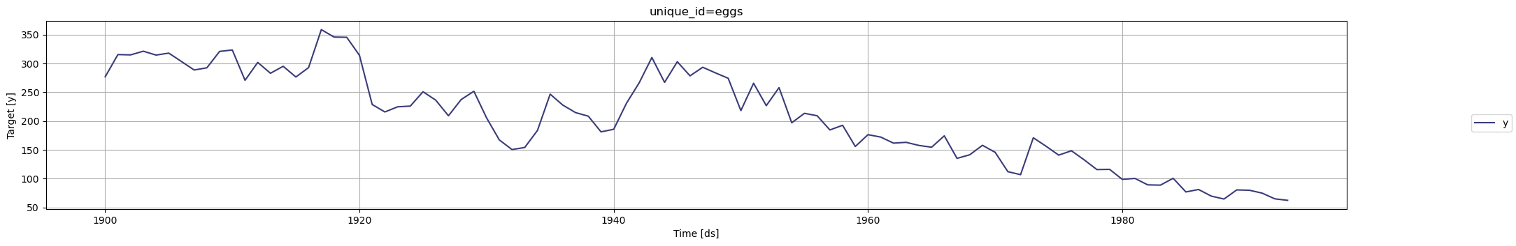
We use the annual egg prices dataset from Forecasting, Principles and Practices. We expect egg prices to be strictly positive, so we want to bound our forecasts to be positive.
Note
You can install
pyreadrwithpip:pip install pyreadr
import pyreadr
from pathlib import Path

# Download and store the dataset
url = 'https://github.com/robjhyndman/fpp3package/raw/master/data/prices.rda'
dst_path = str(Path.cwd().joinpath('prices.rda'))
result = pyreadr.read_r(pyreadr.download_file(url, dst_path), dst_path)
# Perform some preprocessing
df = result['prices'][['year', 'eggs']]
df = df.dropna().reset_index(drop=True)
df = df.rename(columns={'year':'ds', 'eggs':'y'})
df['ds'] = pd.to_datetime(df['ds'], format='%Y')
df['unique_id'] = 'eggs'

df.tail(10)
| ds | y | unique_id | |
|---|---|---|---|
| 84 | 1984-01-01 | 100.58 | eggs |
| 85 | 1985-01-01 | 76.84 | eggs |
| 86 | 1986-01-01 | 81.10 | eggs |
| 87 | 1987-01-01 | 69.60 | eggs |
| 88 | 1988-01-01 | 64.55 | eggs |
| 89 | 1989-01-01 | 80.36 | eggs |
| 90 | 1990-01-01 | 79.79 | eggs |
| 91 | 1991-01-01 | 74.79 | eggs |
| 92 | 1992-01-01 | 64.86 | eggs |
| 93 | 1993-01-01 | 62.27 | eggs |
We can have a look at how the prices have evolved in the 20th century, demonstrating that the price is trending down.
nixtla_client.plot(df)
3. Bounded forecasts with TimeGPT
First, we transform the target data. In this case, we will log-transform the data prior to forecasting, such that we can only forecast positive prices.
df_transformed = df.copy()
df_transformed['y'] = np.log(df_transformed['y'])
We will create forecasts for the next 10 years, and we include an 80, 90 and 99.5 percentile of our forecast distribution.
timegpt_fcst_with_transform = nixtla_client.forecast(df=df_transformed, h=10, freq='Y', level=[80, 90, 99.5])
INFO:nixtla.nixtla_client:Validating inputs...
INFO:nixtla.nixtla_client:Preprocessing dataframes...
INFO:nixtla.nixtla_client:Inferred freq: AS-JAN
INFO:nixtla.nixtla_client:Restricting input...
INFO:nixtla.nixtla_client:Calling Forecast Endpoint...
Available models in Azure AI
If you are using an Azure AI endpoint, please be sure to set
model="azureai":
nixtla_client.forecast(..., model="azureai")For the public API, we support two models:
timegpt-1andtimegpt-1-long-horizon.By default,
timegpt-1is used. Please see this tutorial on how and when to usetimegpt-1-long-horizon.
After having created the forecasts, we need to inverse the transformation that we applied earlier. With a log-transformation, this simply means we need to exponentiate the forecasts:
cols_to_transform = [col for col in timegpt_fcst_with_transform if col not in ['unique_id', 'ds']]
for col in cols_to_transform:
    timegpt_fcst_with_transform[col] = np.exp(timegpt_fcst_with_transform[col])
Now, we can plot the forecasts. We include a number of prediction intervals, indicating the 80, 90 and 99.5 percentile of our forecast distribution.
nixtla_client.plot(
    df,
    timegpt_fcst_with_transform,
    level=[80, 90, 99.5],
    max_insample_length=20
)
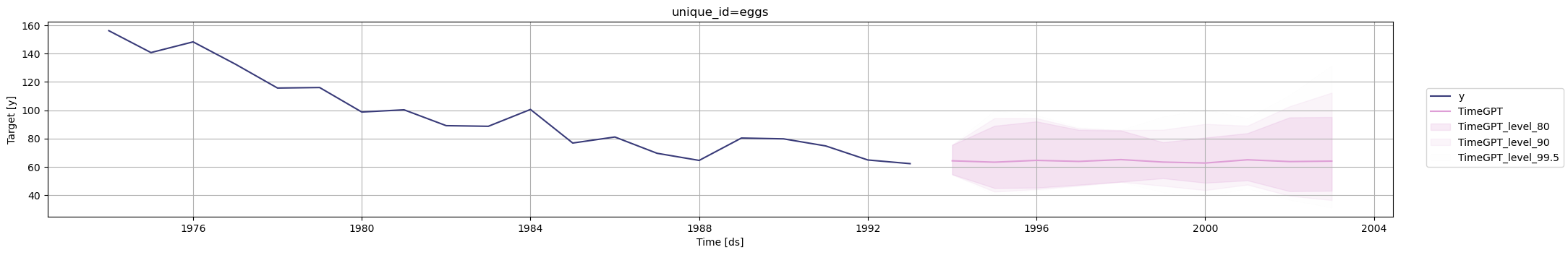
The forecast and the prediction intervals look reasonable.
Let’s compare these forecasts to the situation where we don’t apply a transformation. In this case, it may be possible to forecast a negative price.
timegpt_fcst_without_transform = nixtla_client.forecast(df=df, h=10, freq='Y', level=[80, 90, 99.5])
INFO:nixtla.nixtla_client:Validating inputs...
INFO:nixtla.nixtla_client:Preprocessing dataframes...
INFO:nixtla.nixtla_client:Inferred freq: AS-JAN
INFO:nixtla.nixtla_client:Restricting input...
INFO:nixtla.nixtla_client:Calling Forecast Endpoint...
Indeed, we now observe prediction intervals that become negative:
nixtla_client.plot(
    df,
    timegpt_fcst_without_transform,
    level=[80, 90, 99.5],
    max_insample_length=20
)
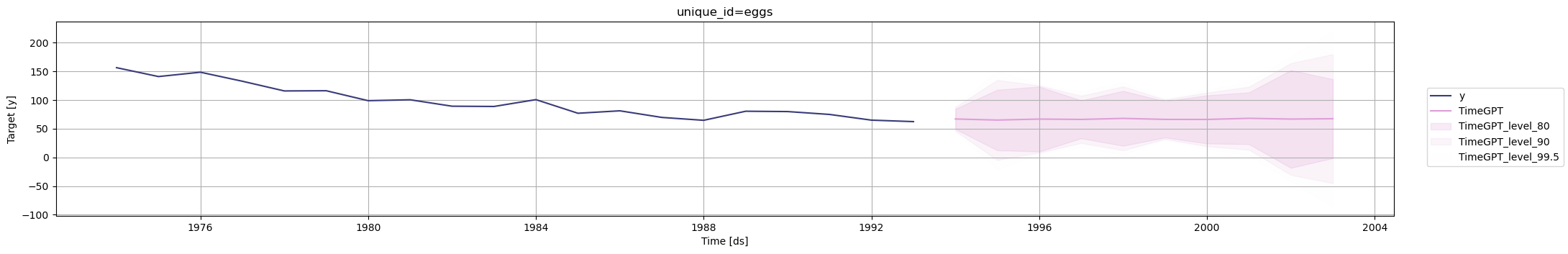
For example, in 1995:
timegpt_fcst_without_transform
| unique_id | ds | TimeGPT | TimeGPT-lo-99.5 | TimeGPT-lo-90 | TimeGPT-lo-80 | TimeGPT-hi-80 | TimeGPT-hi-90 | TimeGPT-hi-99.5 | |
|---|---|---|---|---|---|---|---|---|---|
| 0 | eggs | 1994-01-01 | 66.859756 | 43.103240 | 46.131448 | 49.319034 | 84.400479 | 87.588065 | 90.616273 |
| 1 | eggs | 1995-01-01 | 64.993477 | -20.924112 | -4.750041 | 12.275298 | 117.711656 | 134.736995 | 150.911066 |
| 2 | eggs | 1996-01-01 | 66.695808 | 6.499170 | 8.291150 | 10.177444 | 123.214173 | 125.100467 | 126.892446 |
| 3 | eggs | 1997-01-01 | 66.103325 | 17.304282 | 24.966939 | 33.032894 | 99.173756 | 107.239711 | 114.902368 |
| 4 | eggs | 1998-01-01 | 67.906517 | 4.995371 | 12.349648 | 20.090992 | 115.722042 | 123.463386 | 130.817663 |
| 5 | eggs | 1999-01-01 | 66.147575 | 29.162207 | 31.804460 | 34.585779 | 97.709372 | 100.490691 | 103.132943 |
| 6 | eggs | 2000-01-01 | 66.062637 | 14.671932 | 19.305822 | 24.183601 | 107.941673 | 112.819453 | 117.453343 |
| 7 | eggs | 2001-01-01 | 68.045769 | 3.915282 | 13.188964 | 22.950736 | 113.140802 | 122.902573 | 132.176256 |
| 8 | eggs | 2002-01-01 | 66.718903 | -42.212631 | -30.583703 | -18.342726 | 151.780531 | 164.021508 | 175.650436 |
| 9 | eggs | 2003-01-01 | 67.344078 | -86.239911 | -44.959745 | -1.506939 | 136.195095 | 179.647901 | 220.928067 |
This demonstrates the value of the log-transformation to obtain bounded forecasts with TimeGPT, which allows us to obtain better calibrated prediction intervals.
References
Updated 4 months ago